An Overview of the Properties of Surfaces #

Surfaces are a key aspect in the study in all of mathematics. Abstractions and investigations of these inherently tied to Differential geometry, Algebraic topology, and Lie Algebras. In fact all of Algebraic topology can be thought of as the study of classification of surfaces, and generalizations of this notion. However in this paper we are only going to focus on two-dimensional submanifolds of $\mathbb{R}^3$. That definition requires a certain level of mathematical maturity, but intuitively we can think of a surface as plane that has been stretched, punctured, and twisted into various shapes.

Since a surface in three dimensions is intrinsically is two dimensional, we naturally would only need to two coordinates to uniquely identify a position. This may seem counter intuitive, but remember we currently are on a surface, the Earth. To specify any point on the surface of the earth we only need a longitude and a latitude. Subsequently we can parameterize any surface with two distinct variables.

A constructive example #

To show how this would work we would look at a simple surface, the sphere. First note that the equation for a sphere with radius of one, centered at the origin is just $x^2 + y^2 + z^2 = 1$. Now I can hear you protest, “That isn’t two variables, it is three!”. Well if we let $x = \sin(\theta)cos(\phi)$, $y= \sin(\theta)\sin(\phi)$, and let $z= \cos(\theta)$, you will notice that we parameterized the surface in only two variables $\theta$ and $\phi$. Notice that we transformed our coordinates from Cartesian to spherical. So lets throw this parameterization into a programming environment to see what this would look like.

For this I decided to use the Julia programming languages to view this as it is the easiest way for me to set things up. Here is the code:

using GLMakie

#This is just standard boilerplate 
#This creates a window that handles 60FPS rendering on the GPU

set_window_config!(;
    vsync = true,
    framerate = 60.0,
    float = false,
    pause_rendering = false,
    focus_on_show = false,
    decorated = true,
    title = "Sphere"
)

#Since this is a two-dimensional surface embedded in R^3 we only need two parameters
#The format to populate the parameters is the following
#Starting point, increment, end point

theta = 0:0.01:2*pi
phi = 0:0.01:pi

#This is our parameterization for a Sphere

x = [sin(theta)*cos(phi) for theta in theta, phi in phi]
y = [sin(theta)*sin(phi) for theta in theta, phi in phi]
z = [cos(theta) for theta in theta, phi in phi]

#This defines our colors

GREEN = "#56DB09"
BLUE = "#0738eb"

colors = [GREEN, BLUE]

#This plots the surface

surface(x,y,z, colormap = colors)

This gives us the following:

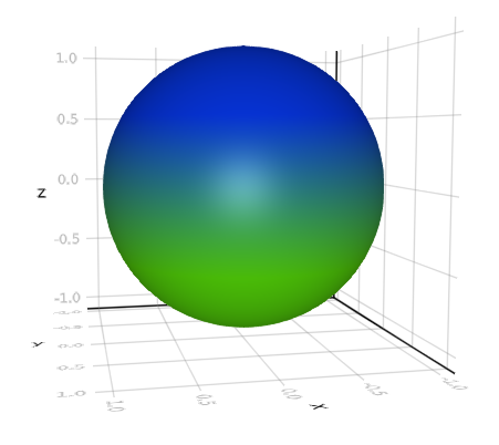
Now keep in mind that this isn’t perfect as certain versions of GLMakie will think that half of the surface is the outside, resulting in a lack of specular mapping.

Minimal Surfaces #

Minimal surfaces arise out of the study of Lagrangian mechanics, and is a central point of study in mathematical physics. Before we get to the formalization lets think of what we mean when we state this. Let us list some example questions that would help us understand how mathematicians came up with the definitions that they have.

• What would a minimal surface be?
• What would it minimize?
• Should it minimize the area of a surface?
• If it minimizes the area, then how do we define this so that a singular point doesn’t satisfy this? It needs to be a surface after all.
• It would make sense that minimal surfaces would arise in nature, since the natural world tries not to waste. If we define something it should appear somewhere in nature.

Ideally a minimal surface should answer all of these questions effectively, but because of the multifaceted nature we should also expect a significant number of equivalent definitions, and as we see in [16], this is true.

The easiest definition is that the mean of its curvatures, its maximal and minimal curvatures, is equal to zero. Assume that our equation is parameterized by two variables $\mathbf{u}$ and $\mathbf{v}$ and the parametric equation of our surface is denoted by $f(u, v)$. It follows then, that each point on the surface has a certain curvature, denoted by the vector, $\vec{\kappa}$ where $\vec{\kappa} = \frac{\mathbf{T}’(t)}{ds}$ where $\mathbf{T}$ is the tangent vector. Thus, by the chain rule, $$\vec{\kappa} = \frac{d\mathbf{T}(t)}{dt}\frac{dt}{ds} = \frac{\frac{d\mathbf{T}}{dt}}{\frac{ds}{dt}} = \frac{\mathbf{T’}}{ \lVert \alpha(t) \rVert } $$ where $\alpha(t)$ is the curve on the surface.

Note that from this definition it is trivial to see that the plane is a minimal surface.

A surface can also be viewed as a minimal surface the surface at any point satisfies the Euler-Lagrange equation.

$$(1 + f_x^2)f_{yy} - 2 f_x f_y f_{xy} + (1+ f_y^2) f_{xx} = 0$$

While the previous is a perfectly fine definition for those who are well acquainted with partial differential equations, and calculus of variations, this justifying this for a surface might to be too much for those who are not mathematically mature. For a more intuitive notion that you can teach to those without the appropriate background, consider the following definition. A minimal surface is just a soap film surface, a continuous surface that a film of soap makes over some wire scaffolding. This is something that makes a lot of sense when you realize that soap films naturally try to minimize the surface, because of the surface tension.

A minimal surface can be any of these as these definitions are all equivalent.

A quick history of minimal surfaces #

Originally the plane was the only minimal surface discovered. If you notice, this trivially satisfies each of the definitions. It was only after extensive study that two surfaces were found to satisfy the definitions, the helicoid and the catenoid. This gave us the first two non-trivial minimal surfaces, but this is less impressive than it first sounds, as the helicoid can be turned into the catenoid through an isometric deformation. In a very real sense the helicoid and the catenoid are the same “type” of shape. However the catenoid has one extra property which is worth mentioning. It and the plane are the only two minimal surfaces that are also surfaces of revolution. This brings us to Scherk’s contribution to minimal surfaces.

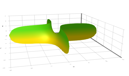
Scherk’s Fifth #

Scherk’s fifth surface, also confusingly known as Scherk’s second surface, was first discovered by Heinrich Ferdinand Scherk, a German mathematician in 1834, while working at University of Kiel [7][12]. Scherk originally was trying to solve a problem posed by French mathematician Joseph Diez Gergonne in 1816, to find a surface with the smallest possible area while still fulfilling certain requirements; for instance bisecting a cube in such a way that the surface of intersection is bound by the inverse diagonals of the opposite faces of the cube. While attempting to solve this problem Scherk managed to become the second person to find a nontrivial minimal surface, and was the first to find a surface that was doubly periodic. Scherk’s work towards this goal did not solve the problem, however he was still awarded a prize for his progress. This was the fifth minimal surface found, and the second minimal surface that Scherk had found.

It is described equally by the following two equations

$$ \sin(z) = \sinh x \sinh y$$

$$f(u,v) = (\sinh^{-1}(u), \sinh^{-1}(v), \sin^{-1}(uv))$$

Analyzing the surface using the tools of Differential Geometry #

If we put a metric on this surface, we can analyze the surface further. A metric, in the realm of geometry, helps defines the properties of a surface. Essentially, it is the relationship between how the curvatures of $\mathbf{u}$ and $\mathbf{v}$ are related at different points on the surface. With knowledge of this relationship, we can deduce certain things about the surface, such as the length of curves, intrinsically and extrinsically. We can also measure the angle between the curvature’s tangent vectors. The metric that is fitted to the surface can be represented by the matrix known as the first fundamental form, which is defined as the following:

On three dimensional surfaces, the coefficients of the first fundamental form are the actual elements used in the metric computations, whereas the metric itself tells how each of those elements interact. A good way to grasp these concepts is to consider yourself a bug on a surface. How you move and the forces you feel are derived from the first fundamental form, and intrinsically manifest in the metric. For the our surface, Scherk’s Fifth, the same logic can be applied. First we must define a parametric form of the equation, and then define what it means to calculate the coefficients $\mathbf{E}$, $\mathbf{F}$, $\mathbf{G}$.

Using the Enneper-Weierstrass parameterization we can parameterize Scherk’s Fifth as the following:

This doesn’t mean much so lets adapt our previous code to look at the shape of it.

using GLMakie

#This is just standard boilerplate 
#This creates a window that handles 60FPS rendering on the GPU

set_window_config!(;
    vsync = true,
    framerate = 60.0,
    float = false,
    pause_rendering = false,
    focus_on_show = false,
    decorated = true,
    title = "Scherk's Fifth"
)

#Since this is a two-dimensional surface embedded in R^3 we only need two parameters
#The format to populate the parameters is the following
#Starting point, increment, end point

r = 0.001:0.001:0.999
theta = 0:0.001:2*pi+0.1

#This is our parameterization for Scherk's Fifth

x = [log((1+ r^2 + 2*r*cos(theta))/(1+r^2 - 2*r*cos(theta))) for r in r, theta in theta]
y = [log((1+ r^2 + 2*r*sin(theta))/(1+r^2 - 2*r*sin(theta))) for r in r, theta in theta]
z = [2*atan((2*r^2*sin(2*theta))/(r^4 -1)) for r in r, theta in theta]

#Theses are just the RGB values for the colors of the surface
#Personally I think these two create a nice contrast against the white background
#The multiple colors allows us to see the contours more easily

YELLOW = "#FFE100"
GREEN = "#56DB09"

colors = [YELLOW, GREEN]

#Finally all we do is call the following function

surface(x,y,z, colormap = colors)

To calculate the first fundamental form, we must find $\textbf{E}$, $\textbf{F}$ and $\textbf{G}$ respectively; where $\textbf{E} = \Phi_r \cdot \Phi_r$, $\textbf{F} = \Phi_r \cdot \Phi_\theta$, and $\textbf{G} = \Phi_\theta \cdot \Phi_\theta$. This results in the coefficients $\textbf{E}$, $\textbf{F}$ and $\textbf{G}$ as follows:

$$\begin{equation} \textbf{E} = \frac{16(1+r^{2})^{2}}{1+r^{8}-2r^{4}\cos(4\theta)} \end{equation}$$

$$\begin{equation} \textbf{F} = 0 \end{equation}$$

$$\begin{equation} \textbf{G}={16r^{2}(1+r^{2})^{2}}{1+r^{8}-2r^{4}\cos(4\theta)} \end{equation}$$

These coefficients can be plugged into the equation $$ds^2 = Edr^2+2Fdrd\theta+Gd\theta^2$$ to determine if the standard notion of the Pythagorean theorem holds on the surface; which in this case obviously doesn’t.

Next lets discuss the second fundamental form. This is also a matrix

Similarly, to calculate the second fundamental form, we must calculate the coefficients for $\textbf{l}$, $\textbf{m}$ and $\textbf{n}$. To do this we must find $\mathbf{U}$ where $$\mathbf{U} = \frac{\Phi_r \times \Phi_\theta}{\lVert \Phi_r \times \Phi_\theta \rVert}.$$

Next we find $\textbf{l}$, $\textbf{m}$ and $\textbf{n}$ such that $\textbf{l} = \Phi_{rr} \cdot \mathbf{U}$, $\textbf{m} = \Phi_{r\theta} \cdot \mathbf{U}$ and $\textbf{n} = \Phi_{\theta \theta} \cdot \mathbf{U}.$ This results in the following coefficients of the second fundamental form’s matrix:

$$\begin{equation} \textbf{l} = \frac{8(1+r^{4})\sin(2\theta)}{1+r^{8}-2r^{4}\cos(4\theta)} \end{equation}$$

$$\begin{equation} \textbf{m} = \frac{8(1-r^{4})\cos(2\theta)}{1+r^{8}-2r^{4}\cos(4\theta)} \end{equation}$$

$$\begin{equation} \textbf{n} = \frac{8r^{2}(1+r^{4})\sin(2\theta)}{1+r^{8}-2r^{4}\cos(4\theta)}\ \end{equation}$$

The Gaussian Curvature for Scherk’s fifth surface also depends on the $r$ and $\theta$, and can be calculated easily once we have generated the first and second fundamental forms. If we define $\textbf{K}$ to be the Gaussian curvature of some surface $\Phi$ then we can simply plug the coefficients of the first and second fundamental form into the following equation: $$\mathbf{K} = \frac{\mathbf{L}\mathbf{N}-\mathbf{M}^2}{\mathbf{E}\mathbf{G}-\mathbf{F}^2 }.$$ This, after careful manipulation simplifies down substantially, yielding: $$\mathbf{K} = -\frac{1+r^{8}-2r^{4}\cos(4\theta)}{4(1+r^{2})^{4}}.$$ Scherk’s surface, is essentially a tower of saddles, and the saddle-like surface is always has a negative Gaussian curvature, and given the pictures of this surface, this makes intuitive sense. If you have a negative curvature throughout a surface, this means that one of the principal curvatures is positive, and the other is negative. Note also that as with every minimal surface the mean of the two principal curvatures is 0.

Uses for Scherk’s Fifth #

Scherk’s surface in engineering

Minimal surfaces in general have a myriad of engineering applications. By the very definition of a minimal surface we quickly can see that they would locally have a minimal mass per unit volume. This is ideal for any applications in fluid dynamics. For example take the heat equation where $u$ is a function determining the heat at any given point on the surface, and $\alpha$ is the thermal diffusivity:

For these applications we can simply treat the surface as some membrane, with a relatively small thickness that we wish to transfer something over. Almost paradoxically heat transfer in gas to fluid interfaces naturally leads to the use of minimal surfaces. To illustrate this first examine the following formula for the force of drag, $$\tfrac12, \rho, A, v^2, C_D.$$ In this equation $\rho$ is the mass density of the fluid, $v$ is the flow velocity relative to the object, $A$ is the cross sectional area orthogonal to the direction of flow, and $C_D$ is the drag coefficient, which can as of this moment not be calculated analytically. From this we can see that if we are trying to maximize some transfer phenomenon between two materials the only thing that we can change is the membrane we are using. We can optimize for $C_D$ however in most of these applications, the direction of the fluid flow through these membranes is unpredictable and essentially random. To optimize for $C_D$ we need to know the velocity of the fluid flow, and the direction at any period of time. Therefore we need a surface that optimizes for $A$ instead, and this obviously leads to a minimal surface.

When we minimize area for any given boundary of a transfer problem, what we are doing is actually minimizing the amount of drag during certain conditions. Also minimizing for area around a boundary allows for thin yet strong structures. This allows us to physically manufacture these at a much smaller level, without the compressive/tensile stress to be as easily limited by the material. The equation for stress on a structure is as follows: $$\sigma =\frac{F}{A}.$$ In this equation $F$ is the force of the load applied and $A$ is the cross sectional area. For any given material the stress that it can handle is some constant, one that is effected by the quality and purity of the material, but still a constant. Note that for drag, the stress is not affected by the area at all. For a minimal surface such as Scherk’s fifth, it has a minimal surface area per unit volume, however it allows fluid flow to circulate through it, and is strong in compression and tension along two intersecting planes. If we subject this surface to a loading orthogonal to these two interesting planes, we can not only maximize strength, but minimize the amount of turbulent flow through the entire structure. The entire structure of Scherk’s surface almost ideal to preserving laminar like conditions of fluid flow throughout the structure. If we tessellate the surface along those planes, we mitigate any discontinuities and maximize the preservation of laminar flow, regardless of the direction of the flow. This combination of minimal turbulence while also being compact and space efficient makes this an ideal candidate for not just volumetrically filling a given space, but also for maximizing any transfer gradient. In fact tessellated Scherk’s surfaces can be used as load bearing items while still performing heat or molecular transfer.

Conclusion #

As we have exhausted all the low hanging fruit associated with the surface, this is a good place to stop. Scherk’s surface is one of a multitude of classified surfaces which over time has influenced mathematical research. Minimal surfaces have far reaching applications previously unforeseen. The simple parameterization associated with it allows it to arise in the study of the natural sciences unexpectedly. This also allows for a myriad of undiscovered engineering applications to exist, just waiting for the taking.

References #

[1] Hoffman, D., & Meeks, W. H. (1990, June). Limits of minimal surfaces and Scherks Fifth Surface. Archive for Rational Mechanics and Analysis, 111(2), 181-195. doi:10.1007/bf00375407

[2] Nguyen, X. H. (2014). Construction of complete embedded self-similar surfaces under mean curvature flow, part III. Duke Mathematical Journal, 163(11), 2023-2056. doi:10.1215/00127094-2795108

[3] Karcher, H., & Polthier, K. (1996). Construction of Triply Periodic Minimal Surfaces. Philosophical Transactions: Mathematical, Physical and Engineering Sciences, 354(1715), 2077-2104. Retrieved from http://www.jstor.org/stable/54581

[4] Oprea, J. (2007). Differential Geometry and Its Applications., 170. Washington, D.C.: Mathematical Association of America.

[5] Peterson, I. (1998). Twists through Space. Science News, 154(9), 143. Retrieved from http://www.jstor.org/stable/4010816

[6] Struik, D. J. (1948). A concise history of mathematics. New York: Dover Publications.

[7] Weisstein, E. M. (n.d.). Scherk’s Minimal Surfaces. Retrieved February 20, 2018, from http://mathworld.wolfram.com/ScherksMinimalSurfaces.html

[8] Scherk surface. (n.d.). Retrieved February 20, 2018, from https://www.encyclopediaofmath.org/index.php/Scherk_surface

[9] Scherk’s Minimal Surface. (2015, November 11). Retrieved February 23, 2018, from https://wewanttolearn.wordpress.com/2015/11/11/scherks-minimal-surface/

[10] Mackay, A. L. (1985). Periodic minimal surfaces. Physica B C, 131(1-3), 300-305. doi:10.1016/0378-4363(85)90163-9

[11] Andersson, S., Hyde, S. T., Larsson, K., & Lidin, S. (1988). Minimal Surfaces and Structures: From Inorganic and Metal Crystals to Cell Membranes and Biopolymers. Chem. Rev., 88(1), 221-242. doi:10.1021/cr00083a011

[12] Heinrich Ferdinand Scherk (1798-1885). (n.d.). Retrieved April 31, 2018, from http://disk.mathematik.uni-halle.de/history/scherk/index.html

[13] Ryan, R. C. (2016). U.S. Patent No. US9440216B2. Washington, DC: U.S. Patent and Trademark Office.

[14] Plateau’s Problem. (n.d.). Retrieved May 9, 2018, from http://mathworld.wolfram.com/PlateausProblem.html

[15] Minimal Surfaces and Soap Bubbles. (n.d.). Retrieved May 10, 2018, from https://math.berkeley.edu/~sethian/2006/Applications/MinimalSurfaces/minimal.html

[16] Pérez, J. (2017). A new golden age of minimal surfaces. Notices of the American Mathematical Society, 64(04), 347–358. https://doi.org/10.1090/noti1500